Multiple Regression in Biology & Analytics

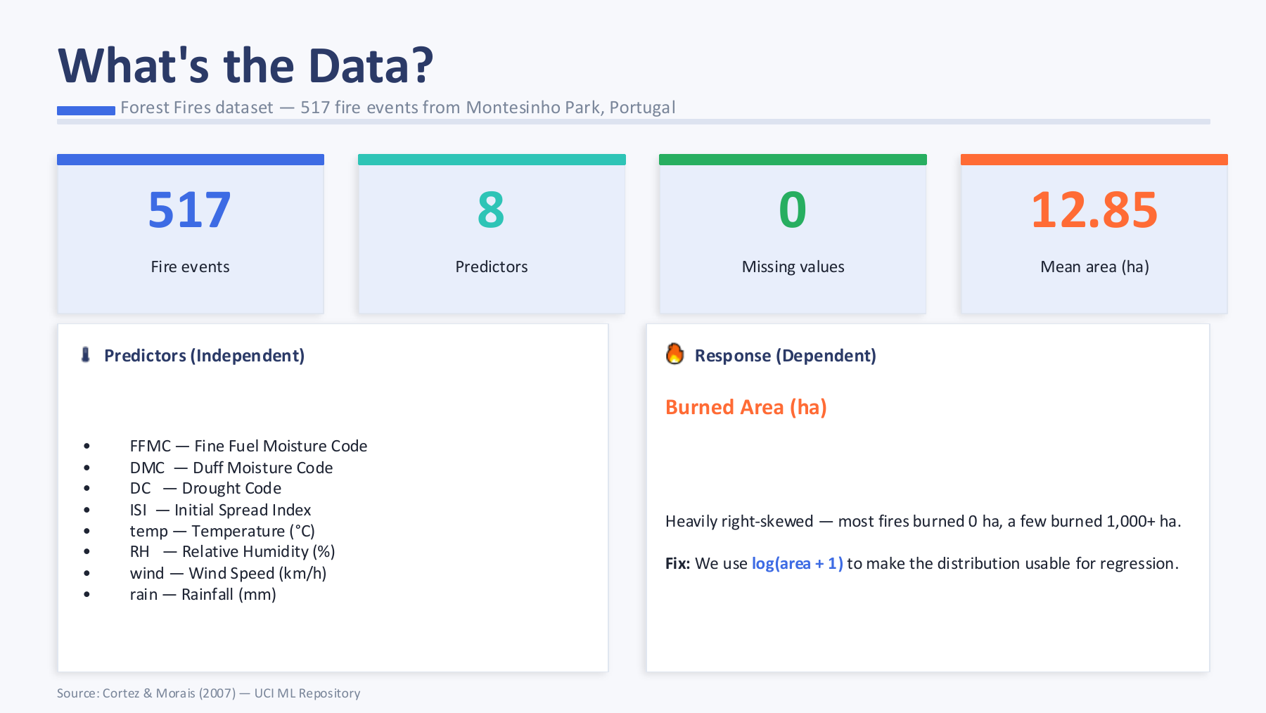
I framed this project around a real analytical tension: forest-fire burned area is not a neat classroom response variable. Most observations are small, a few are extreme, and the process is shaped by weather, fuel moisture, wind, terrain, vegetation, and human response. My job was to use multiple regression carefully without pretending that the available variables could explain the whole ecological system.

The original burned-area variable was heavily right-skewed. The median fire burned only 0.52 hectares, while the maximum reached 1090.84 hectares. I used log(area + 1) to compress extreme values and make the response more workable for OLS. This did not magically make the problem easy, but it made the model more statistically defensible.

The scatterplots showed a pattern that shaped the whole case: the predictors contained signal, but not the kind of clean linear signal that produces a high explanatory model. DMC and DC were strongly related to each other, temperature and humidity moved in opposite directions, and wind showed one of the more useful relationships with log burned area.

The full model included FFMC, DMC, DC, ISI, temperature, relative humidity, wind, and rain. The result was intentionally sobering: adjusted R-squared was only 0.004 and the overall model p-value was 0.247. Wind was the only statistically significant predictor in that model, with beta = 0.0758 and p = 0.039. I treated that as a meaningful but limited finding: higher wind is associated with larger fires, but weather variables alone are not enough to predict burned area well.

I used VIF to test whether multicollinearity was distorting the coefficients. Every VIF was below 5, with the highest value at 2.66 for temperature, so multicollinearity was not the core issue. The Breusch-Pagan test did not reject homoscedasticity, but the Shapiro-Wilk test strongly rejected residual normality. That result made sense because even after transformation, fire outcomes still have heavy tails.

I tested temporal controls, a temperature-humidity interaction, and a stepwise candidate model. Month/day controls raised adjusted R-squared to 0.021, but the improvement was still modest. The interaction term was not significant. Stepwise selection reduced the model to DMC, RH, and wind, with the lowest AIC and BIC among the candidates, but even that model remained practically limited. The important point was not to crown a model too loudly when the data did not earn it.

I used an 80/20 train/test split with caret to check how the model behaved outside the training data. The test-set RMSE was 1.71 and MAE was 1.30 on the log scale. That validation result supported the same conclusion as the regression summary: the model can identify directional environmental influence, but it should not be sold as a precise fire-size prediction engine.

The final takeaway was not that regression failed. It was that the response is complex and the available variables only describe part of the fire process. Wind repeatedly appeared as the strongest predictor, but the low R-squared showed that burned area also depends on missing variables such as slope, vegetation, fuel continuity, ignition location, suppression speed, and spatial spread. I used the model to say something careful, not something exaggerated.

This project is personal to me because it shows the way I want to handle analytics work: I do not just chase a significant coefficient or a beautiful slide. I clean the data, question the assumptions, compare models, validate performance, and then explain the result in language a decision-maker can use. The strongest part of this case is the honesty of the conclusion: weak prediction can still be valuable when it is interpreted with discipline.