Product Demand Time Series Forecasting

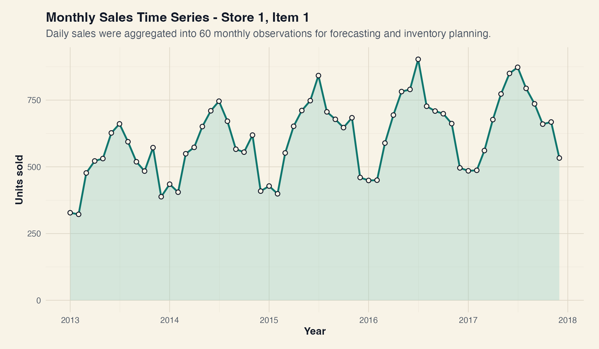
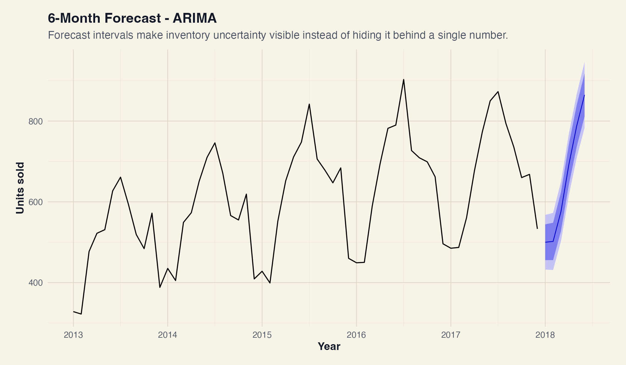
The case starts with a practical operating question: how much demand should the company prepare for next month and the months after that? I framed forecasting as an inventory decision instead of a purely statistical exercise. That kept the model comparison grounded in stockouts, overstock, reorder planning, and the value of forecast uncertainty.

The source training file contained 913,000 daily sales records for 10 stores and 50 items from 2013 to 2017. To keep the case interpretable, I focused on Store 1 and Item 1, then aggregated the daily records into 60 monthly observations. That monthly series became the decision unit for inventory planning.

The series had a clear recurring seasonal shape and a level that changed over time, so I compared additive and multiplicative decomposition before fitting forecasting models. The multiplicative view matched the business pattern better because seasonal swings grew and shrank with the demand level rather than staying fixed in absolute units.

Before fitting ARIMA, I checked stationarity rather than assuming it. The ADF and KPSS results pointed to a series that still needed transformation, so I used first differencing and seasonal differencing. That gave the final ARIMA model a more defensible statistical foundation.

The final comparison was between an ARIMA(0,1,1)(0,1,0)[12] model and an ETS(M,Ad,M) model. ARIMA had the stronger inventory-facing accuracy profile, especially on MAPE, while ETS remained useful as a benchmark because it modeled level, trend, and multiplicative seasonality directly.

The six-month holdout was the credibility check. ARIMA reached 4.46% MAPE, RMSE 38.48, MAE 32.33, and Theil's U 0.403. ETS had slightly lower RMSE, but ARIMA had the better MAPE and Theil's U, which made it easier to defend for percentage-based inventory planning.

The selected ARIMA forecast moved from roughly 500 units in the first month to roughly 865 units by month six. The 95% forecast intervals implied a practical safety-stock buffer around 70 to 80 units per month, with peak months needing the higher end of that range. That translation from uncertainty to buffer stock is where the case becomes operational.

The case uses only historical sales, so it cannot directly adjust for promotions, pricing, holidays, weather, or competitor behavior. It also focuses on one store-item pair and a short forecast horizon. I treated those limits as part of the recommendation: use the model for rolling monthly planning, then extend it later with external drivers and hierarchical forecasting.

This case shows how I connect statistical modeling with a real operating decision. I do not want a forecast to stop at a chart. I want the workflow to explain the data, test the assumptions, compare alternatives, quantify uncertainty, and end with guidance that a team can actually use.